We were able to identify that the average fundamental frequency of the songs from Drake is 57.3. The average fundamental frequency of the songs from Taylor Swift is 52.18. The average fundamental frequency of the songs from Pitbull is 41.631. We didn't use this data, however, as we realized that the fundamental frequencies for each artist varied drastically from song to song, so this data would be of minimal use.

​

​

​

​

​

​

​

 

​

Vocal Isolation

After basic filtering, there was a dual step process we attempted to isolate the vocals. The first is a simple method of subtracting off the left channel of the wav file from the right channel. When a song is decomposed into two channels, it is common to find the vocals in both channels, but the instrumentals heavy in one channel. Subtracting the left channel from the right, in this case, would eliminate most of the vocals due to destructive interference, however it would keep the instrumental. An example of this being used on the song Love Story by Taylor Swift is below.

 

 

 

 

 

Once we had this instrumental version of our song, we attempted to implement our second method, the phase inversion technique. This required us to reverse the phase of the instrumental sample in the frequency domain, then to add the inverted sample back to the original sample in hopes to cancel out the frequency components of the instrumental, leaving just the vocals.

 

As we began to play with the phase inversion technique, it became clear that it was more complex than anticipated, and that it highly depends on the specific song we’re analyzing. This, combined with the fact that not every song in our data set can clearly produce an isolated instrumental by simply subtracting the left channel from the right, means that replicating this process for each individual song for our data set would be too time consuming to be applicable. For filtering, we decided to place a notch filter of the fundamental frequency to filter out some of the more intense instrumentals of the songs. While it is true that for a minority of the songs, the vocals are the strongest frequency component, the instrumental consistently had the most intensity in the songs. This was the filtering we applied to each song before implementing them in the classifier.

​

​

​

​

​

​

​

​

​

​

​

​

Machine Learning

 

Support Vector Machine (SVM):

We attempted using SVM as a second way to classify our audio clips. The idea was that once we classified the songs using the Kth Nearest Neighbor ML algorithm we tried seeing if using an SVM classification as a second step would yield more accurate results. As a proof of concept, we started by directly seeing if SVM would be a viable method to differentiate between two artists of the same gender. We trained 6 clips from both Lana Del Ray and Taylor Swift and used 3 clips from each artist as the test data.

​

Our process in MATLAB was the following:

1. Load the audio files

2. Calculate MFCC coefficients [2] of each song (did 14 per clip)

3. Store the mean value of these coefficients for each song

4. Create our two categories for classification (Artist A: Lana Del Ray, Artist B: Taylor Swift)

5. Use 6 clips from each artist as training data and 3 clips from each artist as test data

6. Standardize features by scaling them to have zero mean and unit variance using z-score normalization

7. Train the linear SVM model using scaled training data

8. Predict the class labels for the test set and evaluate the accuracy

9. Create a heatmap visualization of the confusion matrix

​

​

​

​

​

​

​

​

​

​

​

​

We switched the training and test data using the same audio clips several times. Every time the model had an 83.3% accuracy rate:

​

 

​

​

​

​

​

​

​

​

​

​

​

​

​

We also repeated this process to differentiate between Drake and Pitbull following the same process. This model yielded a 67% accuracy:

​

Ultimately, it was difficult to implement this algorithm with the Kth Nearest Neighbor algorithm under the time constraint. This was an idea we came up with late in our process, but it could be a promising next step to improve our classification accuracy.

​

Decision Tree

We trained three separate decision trees with three datasets for each. For our decision trees, we decided to use 10 samples of songs from each of Drake, Taylor Swift, Pitbull, and Beyonce. The process began with processing our songs and extracting our desired features from each of them. For our first decision tree we used the fingerprints from each of the songs to train our decision tree. The feature we extracted from each song for our second decision tree was the maximum value of the magnitude spectrum (power spectral density) across each time frame. Lastly, we extracted Mel-frequency cepstral coefficients (MFCCs) [2] from each of the songs to train our third decision tree.
 

Decision Tree 1 MATLAB Process:

1. Load the audio files

2. Generate the fingerprints for each song utilizing the method described in the tools section for fingerprinting

3. Create our four labels for classification (Drake, Taylor Swift, Pitbull Beyonce)

4. Set rng seed for reproducibility

5. Use the randperm() function to randomly select 80% of our fingerprints to be used as training data and 20% to be used as test data

6. Train the decision tree using our randomly selected training data

7. Predict the class labels for the test set and evaluate the accuracy

8. Display decision tree viewer

9. Repeats steps 1-8 100 times using different rng seeds 1-100

​

​

​

​

​

​

​

​

​

​

​

​

​

​

​

​

​

​

Decision Tree 2 MATLAB Process:

1. Load the audio files

2. Compute the spectrogram of each song to generate a spectrogram matrix for each song

3. Calculate the maximum magnitude value across time frames for each frequency to generate a feature matrix for each song for the decision tree

4. Create our four labels for classification (Drake, Taylor Swift, Pitbull Beyonce)

5. Set rng seed for reproducibility

6. Use the randperm() function to randomly select 80% of our feature matrices to be used as training data and 20% to be used as test data

7. Train the decision tree using our randomly selected training data

8. Predict the class labels for the test set and evaluate the accuracy

9. Display decision tree viewer

10. Repeats steps 1-9 100 times using different rng seeds 1-100

​

​

​

​

​

​

​

​

​

​

​

​

 

 

 

​

​

Decision Tree 3 MATLAB Process:

1. Load the audio files

2. Extract the 13 MFCCs from each song using the audioFeatureExtractor() function

3. Calculate the mean of each of the coefficients for each of the songs and store them in a 13x1 feature vector

4. Create our four labels for classification (Drake, Taylor Swift, Pitbull Beyonce)

5. Set rng seed for reproducibility

6. Use the randperm() function to randomly select 80% of our feature vectors to be used as training data and 20% to be used as test data

7. Train the decision tree using our randomly selected training data

8. Predict the class labels for the test set and evaluate the accuracy

9. Display decision tree viewer

10. Repeats steps 1-9 100 times using different rng seeds 1-100

 

 

​

​

​

​

​

​

​

​

​

​

​

​

​

​

​

​

​

​

​

The accuracy for Decision Tree 1 was incredibly low. One reason why the decision tree for the fingerprint was so inaccurate was because the decision tree was trying to compare points on the fingerprints with each other. Although fingerprints work well for matching songs that are in a database because each fingerprint is unique to a song, there is not much similarity between each of the fingerprints, so they are not helpful for classifying musical artists.

 

While the results for Decision Trees 2 and 3 showed that this classifier was more accurate than randomly guessing which artist made each song, their accuracy still left much to be desired. An advantage of Decision Tree 2 was that extracting the maximum magnitude value across time frames for each frequency for each song takes a lot less computational time compared to Decision trees 1 and 3. A disadvantage is that it focuses on the dominant characteristics of the song, so if the instrumental section is dominating a song, then it makes it harder to identify the song based on the voice of the artist, which is usually more unique-sounding than drums, for example. An advantage of Decision Tree 3 is that MFCCs provide information about the vocal characteristics of the song, which can make it easier to identify the song based on the voice of the artist. The main disadvantage of using MFCCs is that extracting them is computationally intensive and slow. In order to make decision tree classification more useful for this project, more research would need to be put into identifying features for training the classifier.

​

Discriminant Analysis

Discriminant analysis works by extracting relevant features from audio signals that can distinguish between different artists or classes. It analyzes the means and covariances of these features within each artist's clips that it is trained on to create discriminant functions. These functions essentially define decision boundaries in the feature space, allowing the algorithm to classify new music clips based on their similarity to the learned patterns from each artist. By leveraging statistical relationships between audio features, discriminant analysis can be a valuable tool for identifying and categorizing music clips according to the distinctive characteristics associated with specific artists.

​

Discriminant Analysis Process:

1. Load the audio files and filter them using notch filter

2. Extract the MFCC and Pitch

3. Create our four labels for classification (Drake, Taylor Swift, Pitbull, Lana Del Rey)

4. Standardize the MFCC and Pitch between all training clips

5. Train the discriminant analysis classifier (16 clips per artist)

6. Cross validate to determine validation accuracy

7. Test the classifier on unseen clips (4 per artist) during its training period

8. Create confusion matrix to visualize performance

​

​

​

​

​

​

​

​

​

​

​

​

​

​

​

​

Above is the confusion matrix from using discriminant analysis for four artists. It is obvious it is not accurate as it struggled to identify artists with over 50% accuracy. Which made us not give too much more thought to this classifier.

​

Naive Bayes

Naive Bayes operates by leveraging probabilistic principles. The algorithm estimates the probability distribution of audio features for each artist and assumes that features are conditionally independent given the artist's identity, constituting the "naive" assumption. It calculates the likelihood of observing a set of features given each artist and combines this with prior probabilities of artist occurrence to determine the probability of an artist given the observed features. Naive Bayes is particularly effective when dealing with high-dimensional data, making it suitable for processing various audio features simultaneously. Therefore Naive Bayes utilizes probabilistic reasoning to classify music clips based on the likelihood of certain feature patterns corresponding to specific artists.

​

Naive Bayes Process:

1. Load the audio files and filter them using notch filter

2. Extract the MFCC and Pitch

3. Create our four labels for classification (Drake, Taylor Swift, Pitbull, Lana Del Rey)

4. Standardize the MFCC and Pitch between all training clips

5. Train the naive bayes classifier (16 clips per artist)

6. Cross validate to determine validation accuracy

7. Test the classifier on unseen clips (4 per artist) during its training period

8. Create confusion matrix to visualize performance

​

​

​

​

​

​

​

​

​

​

​

​

​

​

​

​

Above we can see the confusion matrix for naive bayes. This one was far better than discriminant analysis so we were encouraged to see this but still not as accurate as we wanted. Leading us to move onto our final classifier.

​

Kth Nearest Neighbors

Using Kth Nearest Neighbors (KNN), the algorithm operates by considering the proximity of a given music clip's features to those of its k nearest neighbors in the feature space. It relies on a distance metric, in our case the Euclidean distance, to quantify the similarity between feature vectors. The algorithm classifies a music clip by a majority vote from its k nearest neighbors, assigning it to the artist most frequently represented within this neighborhood. KNN is effective in our identification application as it captures local patterns and can adapt well to varying artist styles. However, the choice of the parameter k is critical, influencing the algorithm's sensitivity to noise and overall performance in categorizing music clips based on their proximity to others in the feature space which we quickly found out.

KNN Process:

1. Load the audio files and filter them using notch filter

2. Extract the MFCC and Pitch

3. Create our four labels for classification (Drake, Taylor Swift, Pitbull, Lana Del Rey)

4. Standardize the MFCC and Pitch between all training clips

5. Train the KNN classifier (16 clips per artist)

6. Cross validate to determine validation accuracy

7. Test the classifier on unseen clips (4 per artist) during its training period

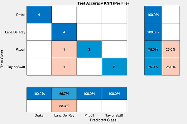
8. Create confusion matrix to visualize performance

​

 

​

​

​

​

​

​

​

​

​

​

​

​

​

​

Above we see the confusion matrix for the KNN classifier. It is easy to see how much better this classifier performed compared to the prior classifier we had used. Which led us to move forward with it as our final models classifier. As we felt we could build off these early results for a strong final model.